

Responsible AI Mitigations and Tracker: New open-source tools for guiding mitigations in Responsible AI
Responsible AI Mitigations: https://github.com/microsoft/responsible-ai-toolbox-mitigations (opens in new tab)
Responsible AI Tracker: https://github.com/microsoft/responsible-ai-toolbox-tracker (opens in new tab)
Authors: Besmira Nushi (Principal Researcher) and Rahee Ghosh Peshawaria (Senior Program Manager)
The goal of responsible AI is to create trustworthy AI systems that benefit people while mitigating harms, which can occur when AI systems fail to perform with fair, reliable, or safe outputs for various stakeholders. Practitioner-oriented tools in this space help with accelerating the model improvement lifecycle from identification to diagnosis and then mitigation of responsible AI concerns. This blog describes two new open-source tools in this space developed at Microsoft Research as part of the larger Responsible AI Toolbox (opens in new tab) effort in collaboration with Azure Machine Learning and Aether, the Microsoft advisory body for AI ethics and effects in engineering and research:
- Responsible AI Mitigations library (opens in new tab) – Python library for implementing and exploring mitigations for Responsible AI.
- Responsible AI Tracker (opens in new tab) – JupyterLab extension for tracking, comparing, and validating Responsible AI mitigations and experiments.
Both new additions to the toolbox currently support structured tabular data.
Throughout the blog, you will learn how these tools fit in the everyday job of a data scientist, how they connect to other tools in the Responsible AI ecosystem, and how to use them for concrete problems in data science and machine learning. We will also use a concrete prediction scenario to illustrate main functionalities of both tools and tie all insights together.
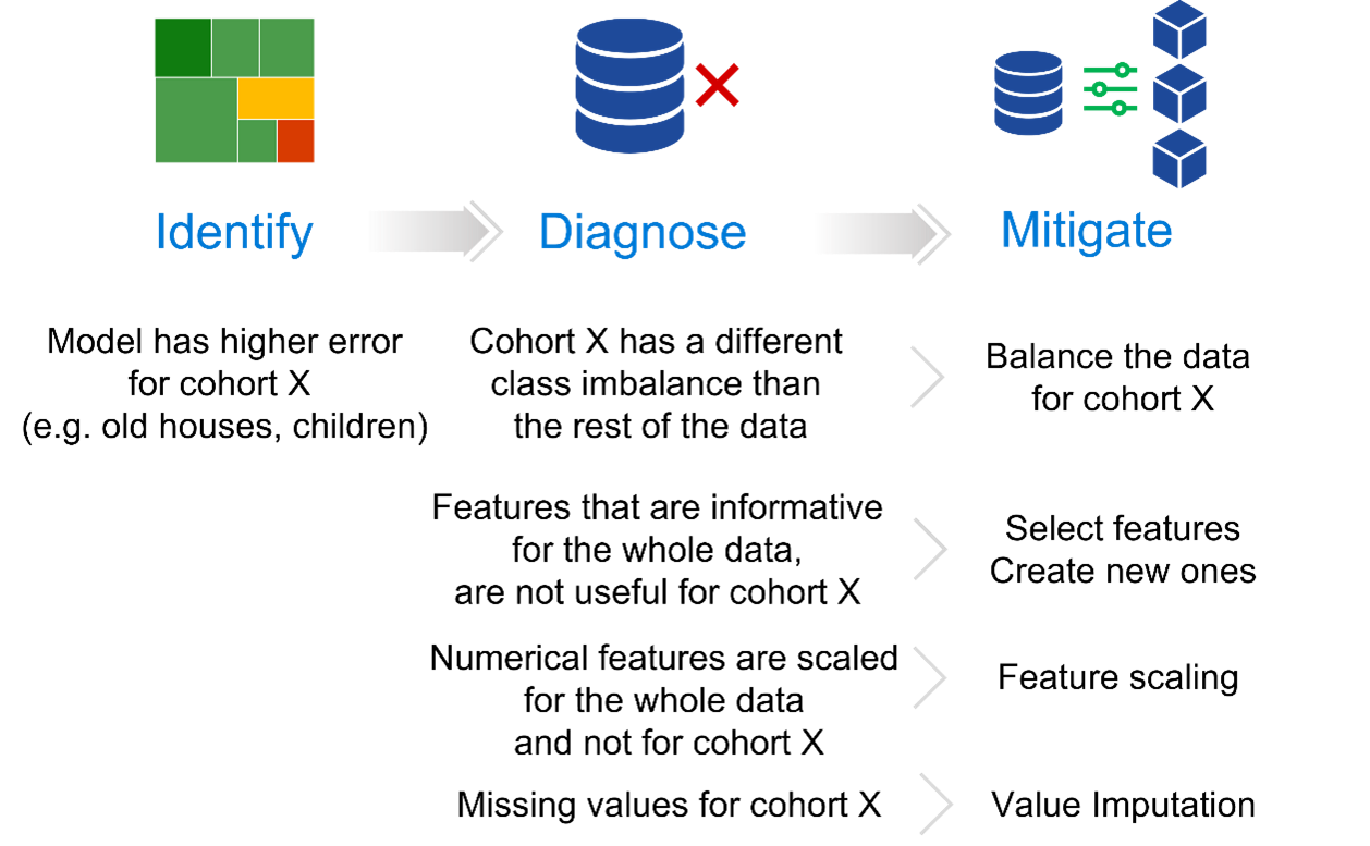
Targeted model improvement
Traditional methods of addressing failures can rely too heavily on a single metric for measuring model effectiveness and approach tackling problems that do arise with more data, more compute, bigger models, and better parameters. While adding more data or compute into the picture as a blanket approach is beneficial, addressing particular problems that negatively impact subsets of the data or cohorts requires a more systematic and cost-effective approach. Targeted model improvement encourages a systematic process of:
- Carefully identifying failure modes during model evaluation.
- Diagnosing factors behind them during model debugging.
- Taking informed mitigation actions during and before model retraining.
- Tracking, comparing, and validating the different mitigation choices during model selection.
In this big picture, the Responsible AI Mitigations library helps data scientists not only implement but also customize mitigation steps according to failure modes and issues they might have found during identification and diagnosis. Responsible AI Tracker then helps with interactively tracking and comparing mitigation experiments, enabling data scientists to see where the model has improved and whether there are variations in performance for different data cohorts. Both tools are meant to be used in combination with already available tools such as the Responsible AI Dashboard (opens in new tab) from the same toolbox, which supports failure mode identification and diagnosis.
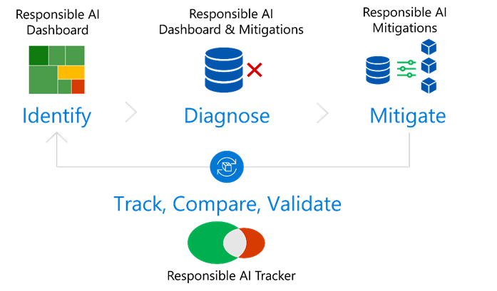
The Responsible AI Toolbox facilitates the process through tools that support each stage.
Next, we show through a data science case study how each of these tools can be used to perform targeted model improvement. For each step we provide code snippets and Jupyter Notebooks that can be used together with the tools.
Case study
Dataset: UCI Income dataset (opens in new tab)
Dataset features: age, workclass, fnlwgt, education, education-num, marital-status, occupation, relationship, race, sex, capital-gain, capital-loss, hours-per-week, native-country
Prediction task: Binary classification. Predicting whether an individual earns more or less than 50K. The positive class in this case is >50K.
Tools needed to run this case study: raimitigations, Responsible AI Tracker extension on Jupyter Lab, raiwidgets
Other libraries: lightgbm, scikit-learn, pandas
Tour notebooks available here (opens in new tab)
Tour video: https://youtu.be/jN6LWFzSLaU (opens in new tab)
Part 1: Identification
Imagine you train a gradient boosting classifier using the LightGBM library and the UCI income dataset. Full notebook available here (opens in new tab).
def split_label(dataset, target_feature):
    X = dataset.drop([target_feature], axis=1)
    y = dataset[[target_feature]]
    return X, y

target_feature = 'income'
categorical_features = ['workclass', 'education', 'marital-status',
                        'occupation', 'relationship', 'race', 'gender', 'native-country']

train_data = pd.read_csv('adult-train.csv', skipinitialspace=True, header=0)
test_data = pd.read_csv('adult-test-sample.csv', skipinitialspace=True, header=0)

X_train_original, y_train = split_label(train_data, target_feature)
X_test_original, y_test = split_label(test_data, target_feature)

estimator = LGBMClassifier(random_state=0, n_estimators=5)

pipe = Pipeline([
    ("imputer", SimpleImputer(strategy='constant', fill_value='?')),
    ("encoder", OneHotEncoder(handle_unknown='ignore', sparse=False)),
    ("estimator", estimator)
])
pipe.fit(X_train_original, y_train)
The overall evaluation of the model shows that the model is 78.9% accurate in the given sample test data, or in other words it makes mistakes for 21.1% of the test data. Before taking any improvement steps, the natural questions for a data scientist would be “Where are most errors concentrated?” and “Are there any cohorts in the data that have a considerably higher error and if so how do these errors map to data or model problems?” Responsible AI Dashboard brings in these insights through disaggregated model evaluation (opens in new tab) and error analysis, fairness assessment, interpretability, and data exploration. Check out this blog (opens in new tab) for a full tour on how to use Responsible AI Dashboard.
For example, this is how you can run the dashboard on this case study:
from raiwidgets import ResponsibleAIDashboard
from responsibleai import RAIInsights
rai_insights = RAIInsights(pipe, train_data, test_data, target_feature, 'classification',
                           categorical_features=categorical_features)
# Interpretability
rai_insights.explainer.add()
# Error Analysis
rai_insights.error_analysis.add()
rai_insights.compute()
ResponsibleAIDashboard(rai_insights)
The dashboard digests the model or predictive pipeline, the training data, and the sample test data. Then it generates insights about input conditions that are main drivers of model errors. Through the dashboard you can find out two major failure modes:
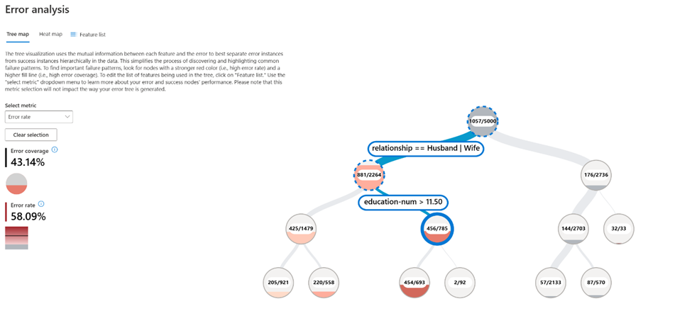
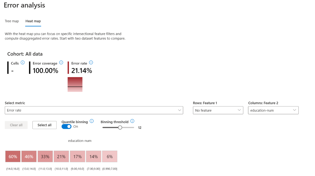
- The error rate increases from 21.1% to 38.9% for individuals who are married.
- The error rate increases from 21.1% to 58.1% for individuals who are married and have a number of years of education higher than 11 (Figure 2). At the same time, we also see that the error rate increases with the number of education years (Figure 3).
Part 2: Diagnosis
Since these cohorts (subsets of the data) seem to have a higher number of errors, we will then see how to further diagnose the underlying problems, mitigate them through the raimitigations library, and continue to track them in Responsible AI Tracker. More specifically, we will track the following cohorts for debugging purposes:
- Married individuals (i.e.
relationship == ‘Wife’ or relationship == ‘Husband’) - Not married individuals (i.e.
relationship <> ‘Wife’ and relationship <> ‘Husband’) - Education > 11 (i.e.
education-num > 11) - Married individuals with Education > 11 (i.e.
(relationship == ‘Wife’ or relationship == ‘Husband’) and (education-num > 11))
When looking at the overall data distribution we see that the ground truth label distribution we see that it is skewed towards the negative class ( <= 50K). However, the cohorts with a higher error have an almost balanced class label distribution, or in the extreme case for married individuals with a number of education years > 11, the skew shifts to the opposite direction with more data where the class label is positive ( > 50K). Given this observation, we can now form the hypothesis that the very different class label distribution and imbalance is the reason behind why the model performs worse for these cohorts.
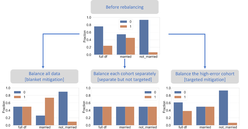
Based on these diagnostics, the immediate question for a data scientist would lead them to investigating data balancing opportunities. However, there may be different ways of balancing the data:
- Balancing all data [blanket mitigation]: This would entail sampling more data for the positive class but not necessarily from the cohorts of interest.
- Balancing each cohort separately [separate but not targeted mitigation]: This would entail sampling more data from the positive class for all disjoint cohorts separately including those that do not have a high error. For simplicity, we will look two disjoint cohorts: “Married” and “Not married”.
- Balancing only the cohort with higher error [targeted mitigation]: This would entail sampling more data from the positive class only for the cohort with higher error (“Married”) and leave the other disjoint cohort as is (“Not married”).
Of course, you could imagine other types of mitigations that are even more customized and targeted, but in this case study we will show that even by only targeting mitigations to the larger “Married” cohort helps other cohorts as well that may also have intersections with this one and that may fail for similar reasons (i.e., different class imbalance than the overall data).
Let’s see how we can implement these situations with the help of the Responsible AI Mitigations library.
Part 3: Mitigations
Formulating and experimenting with targeted model improvements can be complex and time consuming. The Responsible AI Mitigations library (opens in new tab) streamlines this process by bringing together well-known machine learning techniques and adapting them to target model errors that occur in specific cohorts or across all data.
The library surfaces error mitigation methods that can be applied at different stages of model development:
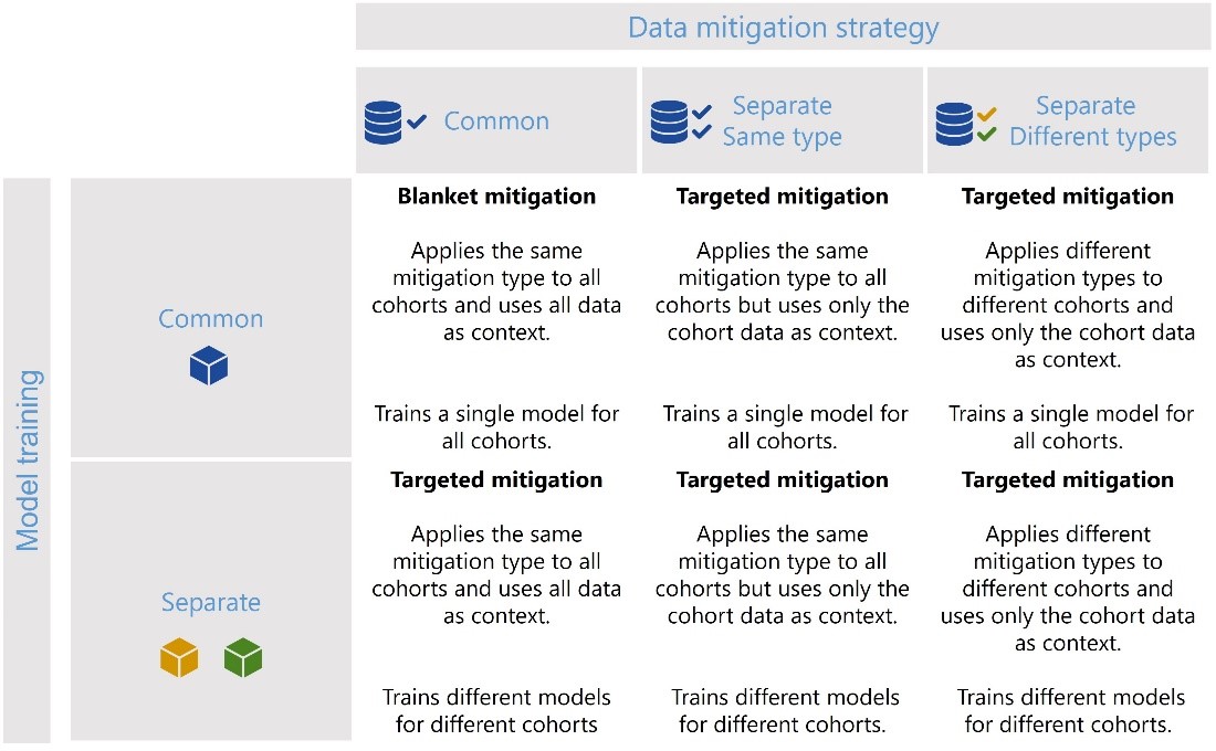
- Data mitigation methods such as data balancing, scaling, and missing value imputation enable transformations of the training data that can improve the resulting model. You will find these mitigations in the DataProcessing (opens in new tab) class of the library. Since different cohorts may have different reasons to why errors happen in the first place (see Figure 5), it is possible to assign different mitigations steps to each cohort, using the CohortManager (opens in new tab) class of the library.
- Model mitigation methods are applied at the time of model training and involves training models separately on data from cohorts where the model is underperforming. This can be achieved by either using the CohortManager (opens in new tab) or the DecoupledClass (opens in new tab) classes in the library.
- Post-training mitigation methods adjust the final model predictions based on custom, automatically found thresholds for each cohort. This can be achieved using the DecoupledClass (opens in new tab) class in the library. The model builds upon prior research work (opens in new tab) proposing post-processing decoupled techniques to improve model fairness.
Using the library, these mitigations can be combined as needed, and applied or customized to specific cohorts for more targeted improvement given different cohorts may have separate issues degrading model performance and benefit from individual mitigations. Figure 6 shows a summary of possible scenarios that can be implemented for targeted mitigations and this notebook (opens in new tab) shows how to implement each of the scenarios.
Beyond surfacing relevant error mitigation methods, the Responsible AI Mitigations library saves time in model development by condensing the code required to explore and test different approaches for improving model performance. For example, without the library support, practitioners would have to split the data manually, apply different mitigations techniques, and then re merge the data making sure that the merge is consistent. The library takes away this complexity and handles all the data splitting and targeted mitigations in the background. By reducing the need for coding custom infrastructure, we aim to allow ML practitioners to focus their time on the modeling problem they are tackling and encourage responsible AI development practices.
Revisiting our case study, we will use the mitigations library to try the mitigations discussed above that may improve the model’s performance. First, you will need to install the raimitigations library from pypi:
pip install raimitigationsBalancing all data
This error mitigation technique involves oversampling from the positive class for all training data. Rebalancing will result in a training dataset with an equal number of instances of the positive and negative class. Retraining with rebalanced data may help address errors from the original model, but this doesn’t guarantee any specific distribution within different cohorts, as can be seen in Figure 7. The following code demonstrates the implementation, also available in this notebook: balance all data.ipynb (opens in new tab). Note that we are leaving out parts of the code that read the data and define the model.
# 24720 is the size of the majority class
rebalance = dp.Rebalance(X=X_train_original, y=y_train,
verbose=False, strategy_over={0:24720, 1:24720})
new_X, new_y = rebalance.fit_resample()

pipe = Pipeline([
    ("imputer", dp.BasicImputer(verbose=False)),

    ("encoder", dp.EncoderOHE(unknown_err=True)),
    ("model", estimator)
])

pipe.fit(new_X, new_y)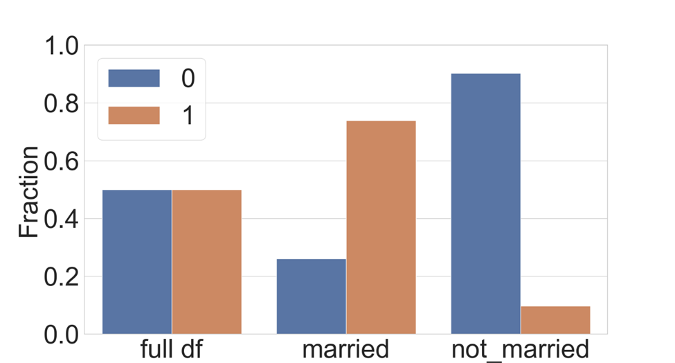
Balancing each cohort separately
A second mitigation strategy we will try is to rebalance the training data again, but do so for each disjoint cohort so that the rebalancing data is sampled from each cohort separately. The assumption here is that resampling only within each cohort will help the model better understand the nuances of class imbalance depending on the cohort. Within each cohort (“Married” and “Not Married” in this case) the rebalanced data will now have the same frequency of positive and negative class examples, as can be seen in Figure 8. The library accepts a transformation pipeline to be specified for each cohort. The following code demonstrates the implementation, also available in this notebook: balance per cohort both.ipynb (opens in new tab). The implementation uses the CohortManager (opens in new tab) class in the raimitigations library, which manages the complexity behind slicing the data, applying mitigations separately, and merging the data again prior to model retraining.
# Define the cohorts
c1 = [ [ ['relationship', '==', 'Wife'], 'or', ['relationship', '==', 'Husband']]]
c2 = None

c1_pipe = [dp.Rebalance(verbose=False,strategy_over={0:24463, 1:24463})]
c2_pipe = [dp.Rebalance(verbose=False,strategy_over={0:16622, 1:16622})]

rebalance_cohort = CohortManager(
    transform_pipe=[c1_pipe, c2_pipe],
    cohort_def={"married":c1, "not_married":c2}
    )

new_X, new_y = rebalance_cohort.fit_resample(X_train_original, y_train)

#Create a pipeline that uses the cohort manager
pipe = Pipeline([
    ("imputer", dp.BasicImputer(verbose=False)),
    ("encoder", dp.EncoderOHE(unknown_err=True)),
    ("model", estimator)
    ])

pipe.fit(new_X, new_y)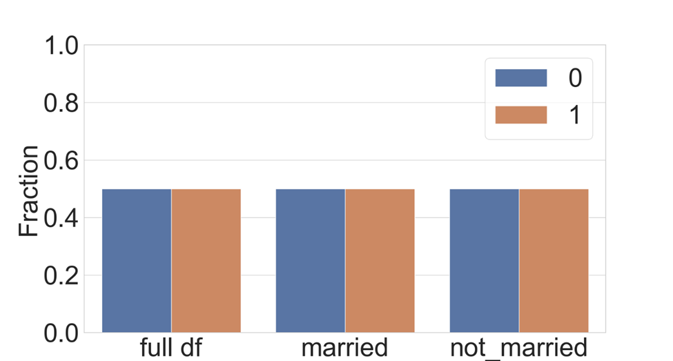
Balancing only the cohort with higher error
The last approach we will evaluate is to perform the rebalance only on the cohort with a high error rate. This targeted mitigation will leave data in other cohorts unchanged while sampling more data from the positive class for the “Married” cohort, as shown in Figure 9. Similar to the previous mitigation, we will specify a transform pipe to rebalance the “Married” cohort, but this time we will give an empty pipeline for the rest of the data. The following code demonstrates the implementation, also available in this notebook: target balance per cohort.ipynb (opens in new tab).
# Define the cohorts
c1 = [ [ ['relationship', '==', 'Wife'], 'or', ['relationship', '==', 'Husband']]]
c2 = None

c1_pipe = [dp.Rebalance(verbose=False,strategy_over={0:24463, 1:24463})]
c2_pipe = []

rebalance_cohort = CohortManager(
    transform_pipe=[c1_pipe, c2_pipe],
    cohort_def={"married":c1, "not_married":c2}
    )

new_X, new_y = rebalance_cohort.fit_resample(X_train_original, y_train)

#Create a pipeline that uses the cohort manager
pipe = Pipeline([
    ("imputer", dp.BasicImputer(verbose=False)),
    ("encoder", dp.EncoderOHE(unknown_err=True)),
    ("model", estimator)
    ])

pipe.fit(new_X, new_y)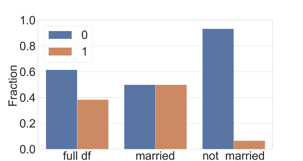
With the three mitigation strategies implemented, we have three new models trained to compare against the original. Next, we’ll discuss how the Responsible AI Tracker can be used to run the comparison and determine which model yields the best results.
Part 4: Tracking, comparing, and validating mitigations
As we saw in the walkthrough for the Responsible AI Mitigations library, during the model improvement lifecycle, data scientists can create several ways of improving the data and the model itself. While some of these improvements yield different rates of overall accuracy improvements, improvement for particular cohorts is not always guaranteed. Performance drops for parts of the data are often referred to as backward incompatibility issues in machine learning. Therefore, it becomes important prior to deployment for practitioners to not only be able to track and compare the different mitigation outcomes, but also validate whether the issues that they were set of addressing on the first place are indeed tackled by the model they would select for deployment.
This is exactly where Responsible AI Tracker (opens in new tab) comes into action. Not only does it enable model comparison across several models and metrics, but it also disaggregates model comparison across cohorts. This fills in a large gap in practice, as this type of functionality is currently not available in most visualizations and the lack of cohort-based comparisons may hide important performance drops.
Responsible AI Tracker is built as an open-source and downloadable extension to Jupyter Lab, the latest web-based interactive development environment for notebooks, code, and data for project Jupyter (opens in new tab). Jupyter Lab has a modular design that invites extensions to expand and enrich functionality. The design has given rise to several fast-growing projects (opens in new tab) in data science to enrich the environment with much needed functionalities.
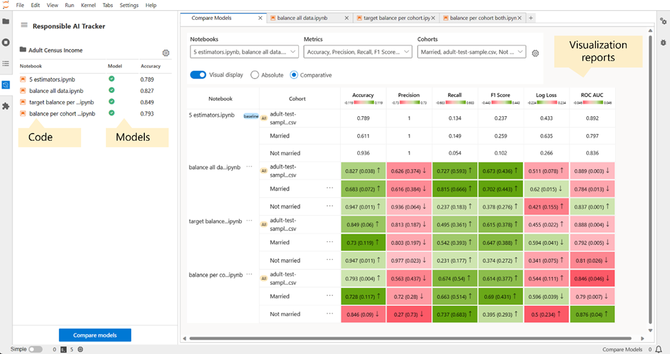
In comparison to Jupyter Notebooks, Jupyter Lab enables practitioners to work with more than one notebook at the same time to better organize their work. Responsible AI Tracker takes this to the next step, by bringing together notebooks, models, and visualization reports on model comparison within the same interface. Practitioners can map notebooks to models such that the relationship between code and models is persisted and tracked easily. The mapping helps with embracing clean data science practices but also accommodates that flexibility that experimental data science still needs to iterate fast through the use of jupyter notebooks.
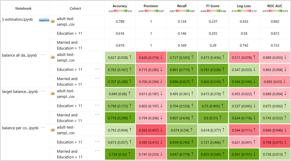
Once a model is registered to a notebook, it then appears in the model comparison table side by side with other models. The model comparison table offers two forms of visualization: absolute and comparative. Generally, it is recommended to use a stronger shade for desirable performance. The absolute view will show raw absolute score metrics and will be shaded using one single color. The comparative view will also show the corresponding differences between model performance and the baseline performance either for the overall dataset or for the given cohort. For example, if the accuracy of the baseline is 0.8 in the overall dataset and the accuracy of a mitigated model is 0.85 for the overall dataset, the respective cell in the table will show 0.85 (0.05 ↑), indicating that there is a 0.05 improvement for the overall dataset. Similarly, if the accuracy of the baseline for the same baseline is instead 0.9 for cohort A, but it is 0.87 for the newly mitigated model, the respective cell for the model and cohort A will show 0.87 (0.03 ↓) indicating a 0.03 decline in accuracy for cohort A. This enables a 1:1 comparison across cohorts over several models. The shading in the comparative view is based on two colors: one for performance improvement (dark red by default) and one for performance decline (dark green by default).
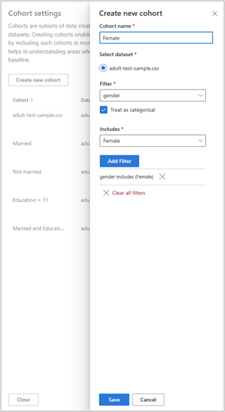
Practitioners can choose which cohorts they want to compare by creating cohorts via the cohort management functionalities. The cohort creation process entails adding one or more filters to the data and saving that cohort for later use in model comparison.
Let’s now go back to our case study and see how the different mitigation ideas we discussed earlier, can be compared and validated.
First, let’s import the four notebooks containing the initial baseline model, along with the notebooks with the data balancing mitigations:
- Initial baseline notebook [only missing value imputation and encoding]: 5 estimators.ipynb (opens in new tab)
- Balancing all data [blanket mitigation]: balance all data.ipynb (opens in new tab)
- Balancing each cohort separately [separate but not targeted mitigation]: balance per cohort both.ipynb (opens in new tab)
- Balancing only the cohort with higher error [targeted mitigation]: target balance per cohort.ipynb (opens in new tab)
Next, let’s run these notebooks and register the corresponding models to the notebooks. The registration process will require the model itself as well as the test dataset (in our case, adult-test-sample.csv (opens in new tab)).).

Then, we can create a few corresponding cohorts of interest to track. In this case, it would be interesting to track the cohorts we had identified at the beginning for comparison:
- Married individuals (i.e.
relationship == ‘Wife’ or relationship == ‘Husband’) - Not married individuals (i.e.
relationship <> ‘Wife’ and relationship <> ‘Husband’) - Education > 11 (i.e.
education-num > 11) - Married individuals with Education > 11 (i.e. (
relationship == ‘Wife’ or relationship == ‘Husband’) and (education-num > 11))
Figure 13 shows how the model comparison table would look like for the “Married” and “Not married” cohorts.
Note on usability: In order to filter and focus on one set of insights at a time, you can also filter the table by notebook, cohort, and metric. Filtering will not only readjust the color shading according to the table content but will also enable you to put relevant numbers side by side, when needed. For example, if you only want to compare model performance on a single cohort, removing all other cohorts from the filter will help with showing all relevant metrics next to each other vertically.

What are the main observations here?
- Balancing all data [blanket mitigation] improves overall model accuracy by ~4% and it benefits both the “Married” and “Not married” cohorts.
- Balancing each cohort separately [separate but not targeted mitigation]: improves overall model accuracy by only 0.4% but it only benefits the “Married” cohort. In contrary, accuracy for the “Not married cohort” drops by 9%. To understand what is happening here, let’s take a look at the training data distribution with respect to class balance before and after each mitigation as shown in Figure 14. Initially, we see that for the “Not married” cohort, the class imbalance is skewed towards the negative class. Rebalancing the data for this cohort, albeit separately (meaning samples are withdrawn only from this cohort), distorts the original prior on this cohort and therefore leads the new model to be less accurate for it.
- Balancing only the cohort with higher error [targeted mitigation] is more effective than the blanket strategy and at the same time does not introduce performance drops for the “Not married” cohort. The approach samples more data with a positive label for the “Married” cohort, without affecting the rest of the data. This allows the model to improve recall for the “Married” cohort and yet keep the prior on more negative labels for the “Not married” one.
In general, we also see that all models sacrifice some of the initial precision for a better recall, which is expected from all such rebalancing strategies.
Finally, Figure 15 also shows how the different models compare with respect to the other cohorts we identified with higher errors at the identification stage. We see that indeed the most problematic cohort (“Married and Education > 11”) is the one that is improved the most, by at least 28%.
Summary
In this extended blog, we saw how a targeted model improvement approach can provide immediate benefits for improving model performance in parts of the data where the model fails the most. The approach is enabled by a set of existing and new tools for Responsible AI: Responsible AI Dashboard (opens in new tab), and most recently Responsible AI Mitigations (opens in new tab) and Tracker (opens in new tab). Looking forward, we hope that such tools will accelerate the process of model improvement and help data scientists and domain experts take informed decisions in the Machine Learning lifecycle. As ML systems and models continue to get deployed in user-facing applications, taking a rigorous and yet accelerated approach to how we build and evaluate Machine Learning will help us create applications that most benefit people and society.
If you have feedback on any of the tools or ideas presented in this blog or would like to propose an open-source collaboration, reach us at rai-toolbox@microsoft.com. All tools described in this blog are open-source and welcome community contributors.
Acknowledgements
This work was made possible through the collaboration of several teams and amazing folks passionate about operationalizing Responsible AI. We are an interdisciplinary team consisting of Machine Learning and front-end engineers, designers, UX researchers, and Machine Learning researchers. If you would like to learn more about the history and journey of this and other work from the team read our hero blog.
Microsoft Research: Dany Rouhana, Matheus Mendonça, Marah Abdin, ThuVan Pham, Irina Spiridonova, Mark Encarnación, Rahee Ghosh Peshawaria, Saleema Amershi, Ece Kamar, Besmira Nushi
Microsoft Aether: Jingya Chen, Mihaela Vorvoreanu, Kathleen Walker, Eric Horvitz
Azure Machine Learning: Gaurav Gupta (opens in new tab), Ilya Matiach (opens in new tab), Roman Lutz (opens in new tab), Ke Xu (opens in new tab), Minsoo Thigpen (opens in new tab), Mehrnoosh Sameki (opens in new tab), Steve Sweetman (opens in new tab)
Big thanks and congratulations to everyone who made this possible!